2 Physics and Perception of Sound

From the outset, it's important to understand that the physics of sound and how we perceive it are not the same. This is a simple fact of biology. Birds can see ultraviolet, and bats can hear ultrasound; humans can't do either. Dogs have up to 40 times more olfactory receptors than humans and correspondingly have a much keener sense of smell. We can only perceive what our bodies are equipped to perceive.

In addition to the limits of our perception, our bodies also structure sensations in ways that don't always align with physics. A good example of this is equal loudness contours. As shown in Figure 2.1, sounds can appear equally loud to humans across frequencies even though the actual sound pressure level (a measure of sound energy) is not constant. In other words, our hearing becomes more sensitive depending on the frequency of the sound.

Figure 2.1: An equal loudness contour showing improved sensitivity to frequencies between 500Hz and 4kHz, which approximately matches the range of human speech frequencies. Image public domain.

Why do we need to understand the physics of sound and perception of sound? Ultimately we hear the sounds we're going to make, but the process of making those sounds is based in physics. So we need to know how both the physics and perception of sound work, at least a bit.

2.1 Waves

Have you ever noticed a dust particle floating in the air, just randomly wandering around? That random movement is known as Brownian motion, and it was shown by Einstein to be evidence for the existence of atoms - that you can see with your own eyes! The movement is caused by air molecules¹³ bombarding the much larger dust particle from random directions, as shown in Figure 2.2.

Figure 2.2: Simulation of Brownian motion. Press Pause to stop the simulation. © Andrew Duffy/CC-BY-NC-SA-4.0.

Amazingly, it is also possible to see sound waves moving through the air, using a technique called Schlieren photography. Schlieren photography captures differences in air pressure, and sound is just a difference in air pressure that travels as a wave. The animation in Figure 2.3 shows a primary wave of sound corresponding to the explosion of the firecracker in slow motion, and we can see that wave radiate outwards from the explosion.

Figure 2.3: Animation of a firecracker exploding in slow motion, captured by Schlieren photography. Note the pressure wave that radiates outward. Image © Mike Hargather. Linked with permission from NPR.

Let's look at a more musical example, the slow motion drum hit shown in Figure 2.4. After the stick hits the drum head, the head first moves inward and then outward, before repeating the inward/outward cycle. When the drum head moves inward, it creates more room for the surrounding air molecules, so the density of the air next to the drum head decreases (i.e., it becomes less dense, because there is more space for the same amount of air molecules). The decrease in density is called rarefaction. When the drum head moves outward, it creates less room for the surrounding air molecules, so the density of the air next to the drum head increases (i.e., it becomes more dense, because there is less space for the same amount of air molecules). The increase in density is called compression.

Figure 2.4: Youtube video of a slow motion drum hit. Watch how the drum head continues to move inward and outward after the hit. Image © Boulder Drum Studio.

You can see an analogous simulation of to the drum hit in Figure 2.5. If you add say 50 particles, grab the handle on the left, and move it to the right, the volume of the chamber decreases, and the pressure in the chamber goes up (compression). Likewise, if you move the handle to the left, the volume of the chamber increases, and the pressure goes down (rarefaction). In the drum example, when the stick hits the head and causes it to move inward, the volume of air above the head will rush in to fill that space (rarefaction), and when the head moves outward, the volume of air above the head will shrink (compression).

Figure 2.5: Simulation of gas in a chamber. Simulation by PhET Interactive Simulations, University of Colorado Boulder, licensed under CC-BY-4.0.

Sound is a difference in air pressure that travels as a wave through compression and rarefaction. We could see this with the firecracker example because the explosion rapidly heated and expanded the air, creating a pressure wave on the boundary between the surrounding air and the hot air. However, as we've seen with the drum and will discuss in more detail later, musical instruments are designed to create more than a single wave. The Schlieren photography animation in Figure 2.6 is more typical of a musical instrument.

Figure 2.6: Animation of a continuous tone from a speaker in slow motion, captured by Schlieren photography. The resulting sound wave shows as lighter compression and darker rarefaction bands that radiate outward. Image © Mike Hargather. Linked with permission from NPR.

The rings in Figure 2.6 represent compression (light) and rarefaction (dark) stages of the wave. It is important to understand that air molecules aren't moving from the speaker to the left side of the image. Instead, the wave is moving the entire distance, and the air molecules are only moving a little bit as a result of the wave.¹⁴

To see how this works, take a look at the simulation in Figure 2.7. Hit the green button to start the sound waves and then select the Particles radio button. The red dots are markers to help you see how much the air is moving as a result of the wave. As you can see, every red dot is staying in their neighborhood by moving in opposite directions as a result of compression and rarefaction cycles. If you select the Both radio button, you can see the outlines of waves on top of the air molecules. Note how each red dot is moving back and forth between a white band and a dark band. If you further select the Graph checkbox, you will see that the white bands in this simulation correspond to increases in pressure and the black bands correspond to decreases in pressure. This type of graph is commonly used to describe waves, so make sure you feel comfortable with it before moving on.

Figure 2.7: Simulation of sound waves. Simulation by PhET Interactive Simulations, University of Colorado Boulder, licensed under CC-BY-4.0.

Now that we've established what sound waves are, let's talk about some important physical properties of sound waves and how we perceive those properties. Most of these properties directly align with the shape of a sound wave.

2.2 Frequency and pitch

Almost all waves we'll talk about are periodic, meaning they repeat themselves over time. If you look at the blue wave in Figure 2.8, you'll notice that it starts at equilibrium pressure (marked as zero¹⁵), goes positive, hits zero again, and then goes negative before hitting zero at 2 seconds. So at 2 seconds, the blue wave has completed 1 full cycle. Now look at the yellow wave. The end of its first cycle is indicated by the circle marker at .5 seconds. By the 2 second mark, the yellow wave has repeated its cycle 4 times. Because the yellow wave has more cycles than the blue wave in the same amount of time, we say that the yellow wave has a higher frequency, i.e. it repeats its cycle more frequently than the blue wave. The standard unit of frequency is Hertz (Hz), which is the number of cycles per second. So the blue wave is .5 Hz and the yellow wave is 2 Hz.

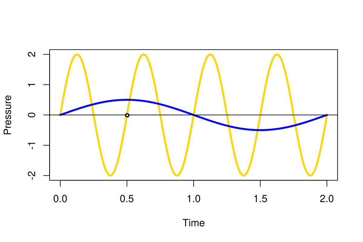
Figure 2.8: Two waves overlaid on the same graph. The yellow wave completes its cycle 4 times in 2 seconds and the blue wave completes its cycle 1 time in 2 seconds, so the frequencies of the waves are 2 Hz and .5 Hz, respectively.

Humans perceive sound wave frequency as pitch. As a sound wave cycles faster, we hear the sound's pitch increase. However, the relationship between frequency and pitch is nonlinear. For example, the pitch A above middle C is 440 Hz¹⁶, but the A one octave higher is 880 Hz, and the A two octaves higher is 1760 Hz. If you wanted to write an equation for this progression, it would look something like \(A_n = 440 * 2^n\), which means the relationship between frequency and pitch is exponential. Figure 2.9 shows the relationship between sound wave frequency and pitch for part of a piano keyboard, together with corresponding white keys and solfège. Notice that the difference in frequencies between the two keys on the far left is about 16 Hz but the difference in frequencies between the two keys on the far right is about 111 Hz. So for low frequencies, the pitches we perceive are closer together in frequency, and for high frequencies, the pitches we perceive are more spread out in frequency.

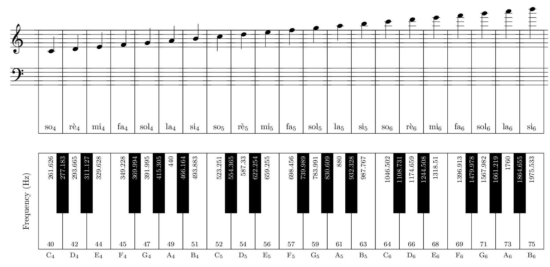
Figure 2.9: Part of an 88 key piano keyboard with frequency of keys in Hz on each key. The corresponding note in musical notation and solfège is arranged above the keys. Zoom in on the image for more detail.

Of course we experience pitch linearly, so the difference in pitch between the two keys in the far left is the same as the difference between the keys on the far right. We can make the relationship linear by taking the logarithm of the frequencies. On the left side of Figure 2.10, we see the exponential relationship between frequency and pitch: as we go higher on the piano keys and pitch increases, the frequencies increase faster, such that the differences in frequencies between keys gets wider. On the right side of Figure 2.10, we see the same piano keys, but we've taken the logarithm of the frequencies, and now the relationship is linear. It turns out that, in general, our perception is logarithmic in nature (this is sometimes called the Weber-Fechner law). Our logarithmic perception of pitch is just one example.

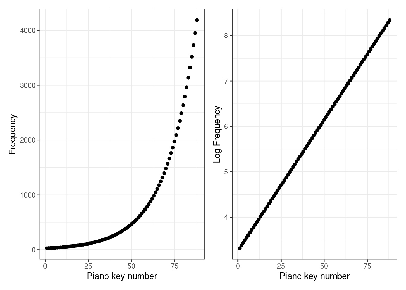
Figure 2.10: (ref:log-freq)

You might be wondering if there's point at which pitches are low enough that the notes run together! It seems the answer to this is that our ability to hear sound at all gives out before this happens. Going back to the 88-key piano keyboard, the two lowest keys (keys 1 & 2; not shown) are about 1.5 Hz apart, but the lowest key¹⁷ is 27.5 Hz. Humans generally can only hear frequencies between 20 Hz and 20,000 Hz (20 kHz). Below 20 Hz, sounds are felt more than heard (especially if they are loud), and above 20 kHz generally can't be heard at all, though intense sounds at these frequencies can still cause hearing damage.

You may also be curious about the fractional frequencies for pitches besides A. This appears to be largely based on several historical conventions. In brief, western music divides the octave into 12 pitches called semitones based on a system called twelve-tone equal temperment. This is why on a piano, there are 12 white and black keys in an octave - each key represents a semitone. It's possible to divide an octave into more or less than 12 pitches, and some cultures do this. In fact, research suggests that our perception of octaves isn't universal either.¹⁸ We'll discuss why notes an octave apart feel somehow the same in a later section.

2.3 Amplitude and loudness

As discussed, sound is a pressure wave with phases of increasing and decreasing pressure. Take a look at the yellow and blue waves in Figure 2.11. The peak compression of each wave cycle has been marked with a dashed line. For the yellow wave, the peak positive pressure is 2, and for the blue wave, the peak positive pressure is .5. This peak deviation of a sound wave from equilibrium pressure is called amplitude.¹⁹ It is perhaps not surprising that we perceive larger deviations (with corresponding large positive and negative pressures) as louder sounds.

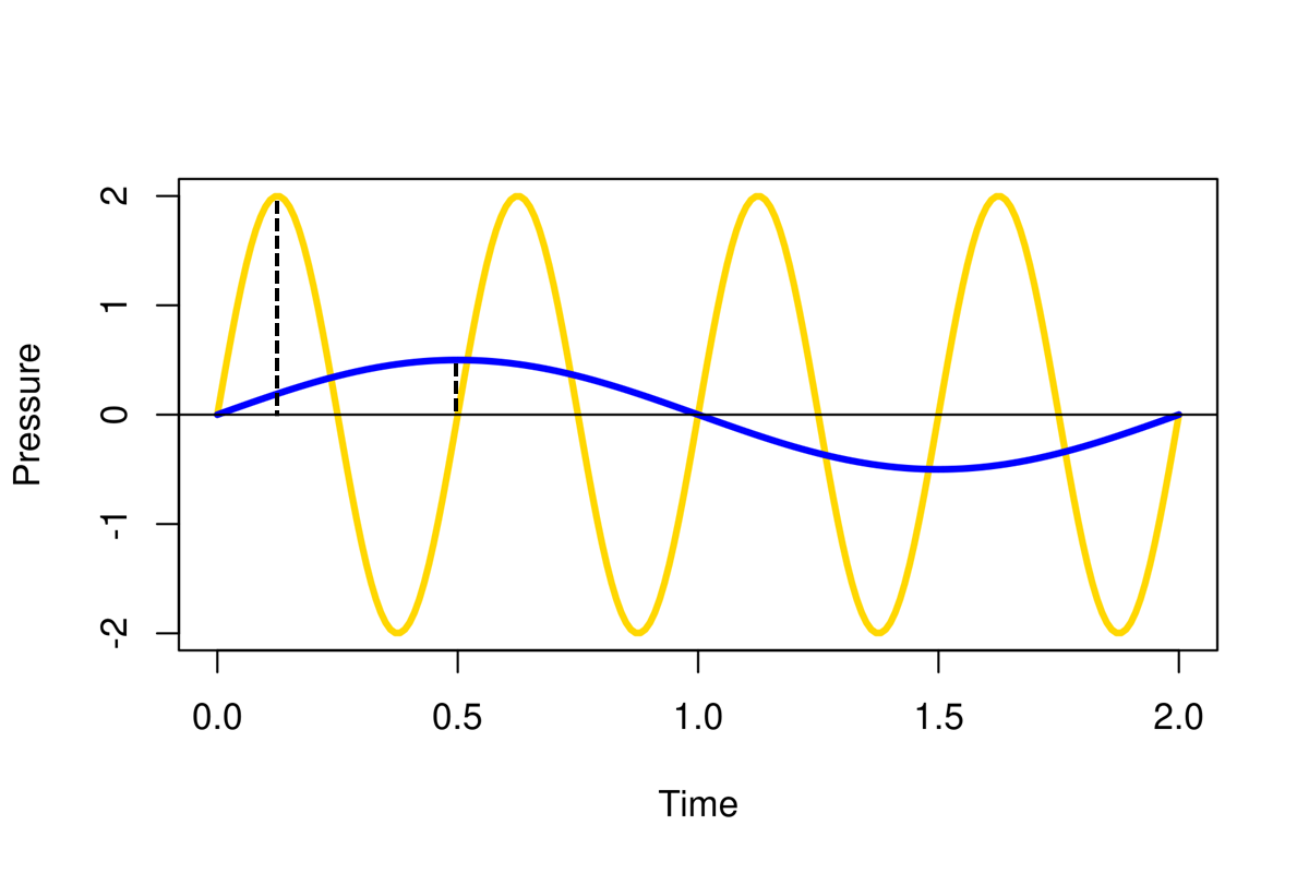
Figure 2.11: Two waves overlaid on the same graph, with a dashed line marking the amplitude of each wave as the deviation from equilibrium.

The relationship between amplitude and loudness is also nonlinear: we hear quiet sounds very well, and sounds must get a lot louder before we perceive them as being louder. In fact, the nonlinear relationship between amplitude and our perception of loudness is even more extreme than the relationship for frequency and pitch.

You might have heard of the unit of loudness before, the decibel (dB). Unfortunately, the decibel is a bit harder to understand than Hz, and it use used as a unit of measurement for different ways of expressing the strength of a sound, like sound pressure, sound power, sound intensity, etc. The most important thing you need to understand about decibels is that they are not an absolute measurement, but rather a relative measurement. Therefore, decibels are always based on a reference value. For hearing, that reference value is the quietest sound people can detect, which is defined as 0 dB. Some examples of 0 to 10dB sounds are a mosquito, breathing, a pin drop, or a leaf hitting the ground.²⁰

If we call the reference sound pressure \(S_0\) and the sound pressure we are measuring \(S\), then we calculate the sound pressure level dB of \(S\) as \(20 * log_{10}(S/S_0)\) dB. Under this definition, a 6 dB increase in sound pressure level means amplitude has doubled: \(20 * log_{10}(2) = 6.02\) dB.²¹ Since our hearing is quickly damaged at 120 dB, you can see that our range of hearing goes from the quietest sound we can hear (0 dB) to a sound that is 1,000,000,000,000 times more intense (120 dB).

Remember from Figure 2.1 that frequency affects our perception of loudness. As a result, we can't say how loud a person will perceive a random 40 dB sound - not in general. One way of approaching this problem is to choose a standard frequency and define loudness for that frequency. The phon/sone system uses a standard frequency of 1 kHz so that a 10 dB increase in sound pressure level is perceived as twice as loud. This relationship is commonly described as needing 10 violins to sound twice as loud as a single violin. There are alternative ways of weighting dB across a range of frequencies rather than just 1 kHz, so the 10 dB figure should be viewed as an oversimplification, though a useful one. Table 2.1 summarizes the above discussion with useful dB values to remember.

Table 2.1: Useful values for working with dB. All values reflect sound pressure or sound pressure level.

Value	Meaning
0 db	Reference level, e.g. quietest audible sound.
6 db increase	Twice the amplitude
10 db increase	Twice as loud
20 db increase	Ten times the amplitude

2.4 Waveshape and timbre

When we talked about frequency and amplitude, we used the same waveshape in Figures 2.8 and 2.11. This wave shape is called the sine wave. The sine wave is defined by the trigonometric sine function and found throughout physics. There are an unlimited number of waveshapes in principle, but in electronic music you will encounter the sine wave and other waveshapes in Figure 2.12 often because they are relatively easy to produce using analogue circuitry.

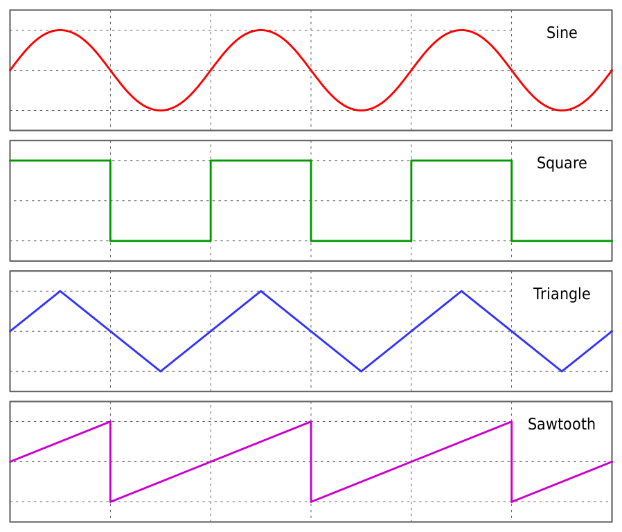
Figure 2.12: The four classic waveshapes in analogue electronic music. Image © Omegatron/CC-BY-SA-3.0.

Perhaps another reason for the widespread use of these waveshapes is that their sounds are rough approximations to real instrument sounds. As we discussed in Section 1.3, the development of electronic music has been strongly influenced by existing instruments. Figure 2.13 presents sounds for each of these waveshapes, together with real instruments that have similar sounds.

As you listen to the waveshape sounds, take a moment to consider their qualities with respect to each other, e.g. how noisy are they and how bright? The differences you're hearing are referred to as timbre or tone color. Each of the waveshape sounds is the same frequency (220 Hz; A3), and the different timbres illustrate how waveforms can have the same frequency but still have their own characteristic sound.

As you listen to the real instrument sounds, consider what about them matches the timbre of the waveshapes and what does not. You may need to listen to some real instruments longer to notice the similarities and differences. For example, when an instrument is played quietly, it may have a different timbre than when it is played loudly. We'll explore these dynamic differences in an upcoming section.

Figure 2.13: Sounds of the four classic waveshapes in electronic music, together with example instruments that make similar sounds.

There is a variation of the square waveform that you will frequently encounter called the pulse wave.²² In a square wave, the wave is high and low 50% of the time. In a pulse wave, the amount of time the wave is high is variable: this is called the duty cycle. A pulse wave with a duty cycle of 75% is high for 75% of its cycle and low the rest of the time. By changing the duty cycle, pulse waves can morph between different real instrument sounds. At 50% they sound brassy, but at 90%, they sound more like an oboe. Figure 2.14 shows a pulse wave across a range of duty cycles, including 100% and 0%, where it is no longer a wave.

Figure 2.14: Animation of a pulse wave across a range of duty cycles. Note that 100% and 0% it ceases to be a wave. Image public domain.

There are multiple ways of creating waveshapes beyond the four discussed so far. One way is to combine waveshapes together. This is somewhat analogous to mixing paint, e.g. you can mix primary colors red and blue to make purple, and we'll get more precise about how it's done shortly. Alternatively, we can focus on what a wave looks like rather than how we can make it with analogue circuitry. Since waves are many repetitions of a single cycle, we could draw an arbitrary shape for a cycle and just keep repeating that to make a wave - this is the essence of wavetable synthesis and is only practical with digital circuitry.

2.5 Phase and interference

The last important property of sound waves that we'll discuss is not about the shape of the wave but rather the timing of the wave. Suppose for a moment that you played the same sine wave out of two speakers. It would be louder, right? Now suppose that you started the sine wave out of one speaker a half cycle later than the other, so that when the first sine wave was in its negative phase, the second sine wave was in its positive phase. What would happen then? These two scenarios are illustrated in Figure 2.15 and are called constructive and destructive interference, respectively. In both cases, the waves combine to create a new wave whose amplitude is the sum of the individual wave amplitudes. When the phase-aligned amplitudes are positive, the amplitude of the resulting wave is greater than the individual waves, and when the phase-aligned amplitudes are a mixture of positive and negative, the amplitude of the resulting wave is less than the individual waves.

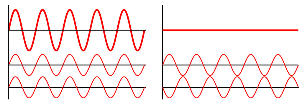
Figure 2.15: Constructive (left) and destructive interference (right). For these matched sine waves, being perfectly in phase or out of phase causes the resulting wave amplitude to be either double or zero, respectively. Image © Haade; Wjh31; Quibik/CC-BY-SA-3.0.

Destructive interference is the principle behind noise cancelling headphones, which produce a sound within the headphones to cancel out the background noise outside the headphones. Figure 2.15 shows how this can be done with with a sine wave using an identical, but perfectly out of phase sine wave. However, being perfectly out of phase is not enough to guarantee cancellation in general. Take a look again at the waveshapes in Figure 2.12. You should find it relatively easy to imagine how the first three would be cancelled by an out of phase copy of themselves. However, the sawtooth wave just doesn't match up the same way, as shown in Figure 2.16.

Figure 2.16: Animation of interference from a perfectly out of phase saw wave (yellow) combined with the original wave (blue). The resulting wave (green) has non-zero amplitude because the out of phase wave does not have opposite amplitude to the original wave at all locations. Dotted lines indicate the positions of the original waves.

Figure 2.16 shows how cancellation will only happen if the perfectly out of phase wave is identical to inverting the original wave. Inverting a wave means reflecting it on the x-axis so we get a mirror image of the wave.²³ When we add a wave to its mirror image, we achieve perfect cancellation, even for waves like the sawtooth. It just so happens that the first three waves in Figure 2.12 are symmetric, which makes their perfect out of phase and and inverted versions identical.

So what is phase exactly? If we consider the cycle of a wave to go from 0 to 1, then the phase of a wave is the position of the wave on that interval. You've likely seen this concept before in geometry with the sine function, where you can describe one cycle either in degrees (360°) or in radians (\(2\pi\)). The unit is somewhat arbitrary: the important thing to remember is that if two waves are out of sync in their cycles, they will interfere with each other, and we describe this difference in cycle position as a difference in phase. The interference caused by phase differences can result in a wide range of effects from cancellation, to the creation of a new wave, to an exact copy of the original wave with double amplitude.

There are a few very practical contexts for phase to keep in mind. The first is that sounds waves reflect, so you don't need two speakers to get phase effects as in the examples above. We'll discuss how phase and reflection are intrinsic to the sounds of many instruments in the next chapter, but any reflective surface can affect phase, which has implications for acoustics in rooms. The second practical context is that you will often want to play multiple notes at the same time, and when you have an electronic instrument, those notes can be triggered very precisely - precisely enough that you have some control over the phase relationships and can use them to shape the sound to your liking.²⁴

2.6 Check your understanding

1. The frequency of the note A one octave above a given A is: double the frequency the square root of the frequency the frequency squared half the frequency

2. What is the standard unit of frequency? Hertz semitones microtones octaves

3. What is the only guaranteed way to achieve phase cancellation? adding a perfectly out of phase wave subtracting a perfectly out of phase wave adding an inverted wave subtracting an inverted wave

4. In Western music, the octave is divided into how many semitones? 8 4 16 12

5. The perceptual correlate of frequency is: loudness timbre pitch

6. The perceptual correlate of amplitude is: pitch loudness timbre

7. A doubling of amplitude is an increase of how many dB? 10 3 20 6