6 Generators
Generators create audible sound. Chapter 4 introduced oscillators, which are the prototypical generator. This chapter expands upon oscillators and how they can be combined together to produce fuller and more interesting sounds. Additionally, two new generators are introduced, noise and samplers. Noise can also be combined with oscillators and other generators to create richer and more realistic sound. Samplers represent the extreme of realism in generators, at least as far as their digital representation allows.
6.1 Chords
Section 3.1 briefly mentioned the relationship between harmonics and fundamental relationships like octaves and fifths. To recap, the second harmonic has double the frequency of the first and so is one octave above the first harmonic. We can express this relationship as 2:1, i.e. an octave is twice the frequency of the the fundamental. Similarly the third harmonic is a fifth above the second harmonic, so we can express a fifth as 3:2.50
Now consider what happens if two notes an octave apart or a fifth apart are played at the same time. Clearly some of their harmonics will be the same. Thus playing two or more notes this way will add and enhance harmonics beyond that of a single note, creating a richer and fuller sound. Of course, notes may be played that are not harmonically related, to a different effect.51 When two notes are played simultaneously, it is called an interval, with three notes, a trichord, with four notes, a tetrachord, etc. Many harmonically related notes can be played simultaneously to good effect. For example, the THX Deep Note in Figure 6.1 resolves to 11 notes, mostly harmonically related by 3, 4, and 7 semitones (minor/major thirds and fifths).
Figure 6.1: Youtube video of the THX Deep Note, which resolves to 11 harmonically related notes. Image © THX Ltd.
In modular synthesis, there are at least two ways to create chords, which correspond to stages of the process to create a single note. At the first stage, we have a V/Oct control signal, so we can create chords by making new control signals harmonically related to the original signal. At the final stage, we have an audio signal, so we can create chords by making new audio signals harmonically related to the original signal. Let's look at both.
To create harmonically related control voltage signals, we can use a voltage offset module to create new signals offset from the original signal, i.e. the original voltage plus/minus a harmonically-related voltage. It can take a little math to do this if the offset module is labeled in volts52, but if the offset module is labeled in semitones, it is fairly straightforward, e.g. a fifth is seven semitones. Additionally we will need multiple oscillators to play a note for each offset voltage. We could reasonably do this with separate oscillators, but some chord-oriented modules contain multiple oscillators and take separate V/Oct for each. Try making a trichord using a fifth and an octave using the button in Figure 6.2.
Figure 6.2: Virtual modular for making a chord using signal offsets.
To create harmonically related audio signals, we can use a clock divider as long as the original signal can be interpreted as clock and the clock divider in question can accept audio rates. This approach is related to a classic technique for creating a fatter sound, the sub-octave square wave. A sub-octave square wave is exactly that: a square wave one octave below the fundamental. Since a clock division of \(/2\) cuts the source clock frequency in half, we can easily generate a sub-octave square wave using a clock divider, albeit with the same assumptions. Perhaps more interestingly, if our clock divider supports both even and odd divisions we can create subharmonic chords, or perhaps more appropriately, an inverted chord. All that is required is knowing the harmonic ratios mentioned above, e.g. 3:2 means that the divisions \(/3\) and \(/2\) are a fifth apart. Try making a trichord using a fifth and an octave using the button in Figure 6.3.
Figure 6.3: Virtual modular for making a chord using clock divisions.
6.2 Chorus
We can also combine different oscillators using the same, or almost the same pitch. As discussed in Section 3.1, two identical waves will constructively interfere with each other and produce a new wave with twice the amplitude. However, if the waves are slightly out of phase or have slightly different frequencies, a subtle interference pattern will be produced that slowly changes the amplitude and timbre of the sound over time. This effect is used in pianos, which have more than one string for most notes, as well as 12-string guitars that have six pairs of identical strings. In fact, this effect is so general is used as an audio processing effect called chorus.
To achieve this effect in modular, one only needs to slightly detune one of the VCOs with respect to the other or change the phase relationship between oscillators. Typically two independent oscillators will already be out of phase, but in modules that contain multiple oscillators there is sometimes a control to adjust the phase of one oscillator with respect to the others. Both detuning and phase changes must be subtle in order to increase the richness of the sound. If the detuning is too great, two different pitches will be perceived as out of tune rather than a richer single sound. Similarly, as phase is increased there is greater destructive interference and potentially cancellation when completely out of phase. Remember that most interference will create spans of sound with greater loudness and quietness, as shown as shown in Figure 6.4.
Figure 6.4: Animation of interfering sine waves as one increases in frequency. Note how multiple beats appear in this short span as the frequency increases. Image © Adjwilley/CC-BY-SA-3.0.
These changes in volume can be perceived as beats if they are strong enough and occur within a certain range of frequencies. Typically such beats are unwanted, so the interference between the sound waves should either be too slow/fast to be perceive as beats or the beats themselves are so soft that they are not perceived as beats. Returning to the first patch, try to detuning the oscillator a fifth above the root while silencing the oscillator an octave above, using the button in Figure 6.3. You should hear a beat whose beat increases as you increase detuning.
Figure 6.5: Virtual modular for detuning a second oscillator.
6.3 Low frequency oscillators & uses
Low frequency oscillators (LFOs) are modules that produce waves at frequencies below audio rates. It may seem strange to introduce LFOs in a chapter on generators, which by our definition create audible sound. The reason is that LFOs are essentially identical to regular oscillators (VCOs) except that LFOs operate at lower frequencies. In fact, it's common to find LFOs that can operate at audio rates and VCOs that operate below audio rates. One other common difference is that LFOs often have a unipolar switch. The switch changes the output of the LFO, which are by default bipolar and range from -5 to +5 V, to unipolar output of 0 to 10 V. We've already met a unipolar LFO by another name - a clock is a unipolar LFO that uses a pulse wave!
LFOs have many potential uses, but perhaps the most prominent is to add movement to a sound. For example, it's generally thought that chorus adds to sound through movement, specifically movement caused by interference and changing harmonics. LFOs can create similar movement in other contexts as described below. What all these contexts share is two properties: the speed of the movement (frequency) and the depth of the movement (amplitude).
6.3.1 Pulse width modulation
LFOs can create the effect of two interfering oscillators with only one VCO. This is an interesting effect in its own right, but is particularly valuable when only one VCO is present. The prototypical case for this effect is with pulse waves, where it is called pulse width modulation (PWM). As a motivating example, consider Figure 6.6, which shows the interference of two pulse waves at 25% and 50% duty cycles, respectively. The resulting wave looks like the 25% wave where the wave is positive and like the 50% wave where the wave is negative. This occurs because the two component waves, which have the same amplitude, combine to either exactly double the amplitude or sum to zero at all points of the wave.
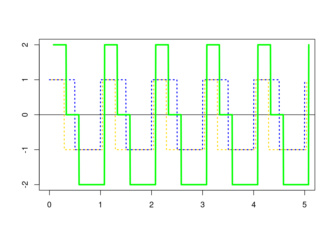
Figure 6.6: Interference of a pulse wave with 25% duty cycle (gold) with a pulse wave with a 50% duty cycle (blue). Note the resulting wave (green) has a positive signal matching the 25% wave and a negative signal matching the 50% wave. Waves are offset for comparison.
Because this is such a useful and interesting effect, many oscillators that produce pulse waves have a PWM input that allows the duty cycle of the wave to be controlled by another module. Try to implement PWM with an LFO using the button in Figure 6.7. If you hook up the VCO square wave to a scope, you can see the resulting waveshape. The LFO frequency and the PWM depth knobs give control over the speed of the PWM and the depth (i.e. the range of duty cycles covered), respectively. As you listen to the result of PWM, take note of the changes in the harmonics. Square waves have only odd harmonics, but pulse waves more generally have every nth harmonic removed, where n is the denominator of the duty cycle of the wave. For example, a square wave with a 50% duty cycle (1/2) has every 2nd harmonic removed, a pulse wave with a 33% duty cycle (1/3) has every 3rd harmonic removed, and so on. Therefore PWM, by modulating the duty cycle, is continuously adding and removing harmonics as the duty cycle changes.
Figure 6.7: Virtual modular for implementing pulse width modulation (PWM) using a low frequency oscillator (LFO).
6.3.2 Vibrato
Vibrato is movement around pitch that can be defined in terms of speed of movement around a center pitch and depth of movement, or distance from, that same center pitch. Vibrato is widely used in music, but is perhaps most strongly associated with opera as shown in Figure 6.8.
Figure 6.8: Youtube video of an opera singer's vibrato, or frequency variation around a central note. Image © jiggle throat.
LFOs can create vibrato on a VCO by controlling V/Oct. Unlike PWM, an additional VCA is needed to control the depth of the vibrato.53 Try to create vibrato with an LFO using the button in Figure 6.9. With a little adjustment of the parameters, it's possible to match the vibrato of the opera singer just discussed. Since no vibrato occurs when the LFO frequency is zero, one can turn the vibrato effect on and off by setting LFO frequency, e.g. through a sequencer.
Figure 6.9: Virtual modular for implementing vibrato using a low frequency oscillator (LFO).
6.3.3 Tremolo
In electronic music, tremolo is movement around loudness that can be defined in terms of speed of movement around a center volume and depth of movement, or distance from, that same center volume.54 Note that in other forms of music, there are different definitions of tremolo. Tremolo has been widely used in popular guitar music since the 1960's, and guitar pedals producing tremolo effects as shown in Figure 6.10 are quite common today.
Figure 6.10: Youtube video of a tremolo guitar pedal. The flashing light corresponds to the speed of loudness changes around a center volume. Image © CheaperPedals.com.
LFOs can create tremolo by controlling the amplitude of VCO output. A VCA is is used to the depth of the tremelo. However, there are two differences with respect to previous patches. First, a VCA accepts unipolar control CV, so the LFO must be set to unipolar. Second, when the LFO goes to zero, it will completely close the VCA just like an envelope does. In order to keep some base line of loudness, you must mix a copy of the VCO output with the tremolo-modified VCO output. Try to create tremolo with an LFO using the button in Figure 6.11 and adjust the parameters to match the tremolo of the guitar pedal in Figure 6.10. As before, no tremolo occurs when the LFO frequency is zero, so on can turn the tremolo effect on and off by setting LFO frequency using a sequencer or other means.
Figure 6.11: Virtual modular for implementing tremolo using a low frequency oscillator (LFO).
6.4 Synchronization
Techniques that allow you to remove/reduce phase relationships between oscillators are called synchronization (sync). Despite seeming contradictory to the preceding discussion, sync can create interesting effects exactly because phase relationships have been removed/reduced. The basic idea of sync is quite simple. Every oscillator has an internal reset trigger that tells it when to start drawing its waveshape again. A sync signal overrides this internal trigger, so we can control when the reset happens.
The most common form of sync is known as hard sync. In hard sync, the sync signal removes phase by forcing an immediate reset. Typically the sync signal is the wave output of one oscillator (the leader), which is connected to the sync input of another oscillator (the follower). If the two waves were identical in frequency, hard sync would simply align them in phase; however this is rarely the case. When the two waves are different in frequency, one wave is reset and therefore has a sharp edges in its waveshape. As discussed in Section 3.2, sharp edges contribute higher partials Sync therefore changes the harmonic content of a wave in a different way than chorus type effects. Notably, the closer the follower's frequency is to an integer multiple of the leader's frequency, the more the sync will emphasize the harmonics of the leader, but in general the new partials will not be harmonically related to the leader. An example of hard sync is shown in Figure 6.12, where the two sine waves on the left are hard synchronized on the right.
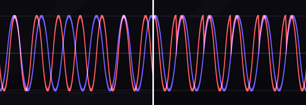
Figure 6.12: An example of hard sync using two sine waves. On the left, the sine waves are not synchronized. On the right, the leader's sine output is connected to the follower's sync input. As soon as the leader's sine wave (blue) increases above zero, the follower's sine wave (red) resets and begins its cycle again, creating a sharp edge in its waveshape.
There are several variations of sync known as soft sync, but they all attempt to align the two oscillators in phase without creating the sharp edge found in hard sync. One notable form of soft sync is reverse soft sync (or flip soft sync). Reverse soft sync reverses the direction of the wave at the moment of reset. This causes the follower to match the direction of the leader without exactly matching the leader's phase. An example of reverse soft sync is shown in Figure 6.13, where the two sine waves on the left are soft synchronized on the right.
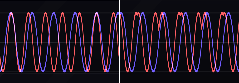
Figure 6.13: An example of reverse soft sync using two sine waves. On the left, the sine waves are not synchronized. On the right, the leader's sine output is connected to the follower's sync input. As soon as the leader's sine wave (blue) increases above zero, the follower's sine wave (red) reverses, i.e. runs in the opposite direction, and begins its cycle again, creating a less sharp edge in its waveshape than hard sync.
Try to create hard and soft sync using the button in Figure 6.14 and that matches Figures 6.12 and 6.13, respectively. Each type of sync produces a characteristic sound that depends on the waveshapes involved and their relative frequencies.
Figure 6.14: Virtual modular for implementing hard and soft sync.
6.5 Noise
Noise is commonly used in synthesis to complement other sounds. As discussed in Section 3.3, there are many different kinds of noise that can be distinguished by the frequencies they emphasize. In modular, noise is typically provided by specialized modules, with separate jacks for different colors of noise.
Noise blended with other generators can create transients and complementary sounds that produce more realistic percussion. For example, a kick drum has an initial noise transient that quickly dies out, and a snare has a long-lasting noise component that comes from the metal snares below the bottom membrane. However, the kick drum noise is tilted towards lower frequencies (e.g. red noise) and the snare is tilted towards higher frequencies (e.g. blue noise). Try to create kick and snare drums with noise using the button in Figure 6.15. The patches are identical except for different noise sources and knob settings.
Figure 6.15: Virtual modular for adding noise to kick and snare drums.
6.6 Samplers
Samplers are popular type of generator that can be used to produce very realistic sounds but simply playing back prerecorded sounds. Samplers are thus very useful for performing with sounds that are difficult to synthesize (e.g. speech) or when it is impractical to use modules to synthesize multiple instruments due to cost/space constraints (as is often the case with percussion).
Samplers do not perform synthesis per se, though there are crossovers like wavetable synthesis, as discussed in Section 2.4. Instead, samplers represent audio data, typically digital audio data, without representing the process that generated the data. Digital audio data is represented according to two parameters that each can be considered a kind of resolution, as shown in Figure 6.16.
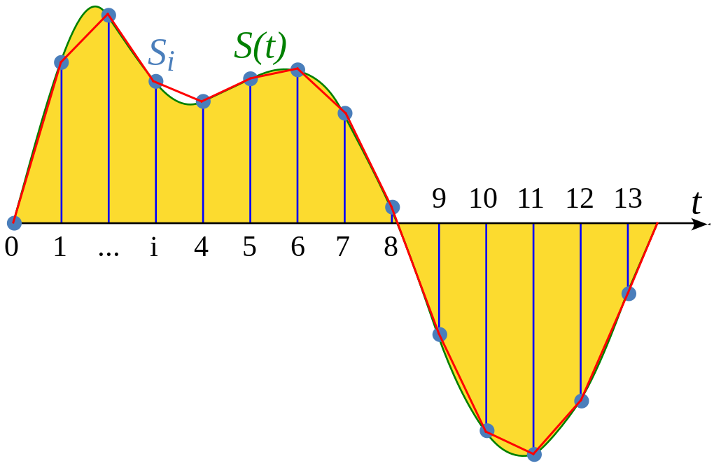
Figure 6.16: A wave digitized by sampling. The sampling rate corresponds to the distance between sample times on the horizontal \(t\) axis. The bit depth corresponds to the accuracy of distance between the axis and sampled points on the wave. The straight red segments are the digital reconstruction of the original wave based on the samples. Image public domain.
Sampling rate measures how close together each sample is taken. If the distance between the samples is small, a straight line is a good approximation of the curve of the wave, and the digital representation has good fidelity to the original sound. However, if frequency of the wave is high or the wave otherwise changes suddenly, those changes may be between samples and not show up in the digital representation at all. Common sample rates are 8 kHz (phone quality), 16 kHz (speech recognition quality), and 44.1 kHz (CD quality).
Why sample at 44.1 kHz when the upper limit of human hearing is around 20 kHz? The 44.1 kHz rate is the Nyquist rate for 22,050 Hz, i.e. the Nyquist rate is double that frequency, which is about 2 kHz above the standard human limit.55 The reason to sample at twice the highest frequency is pretty simple. If we assume all sounds are made of sine waves, as covered in Section 3.2, then we need to be able to define the highest frequency component in our audio as a sine wave. If we evenly sample at least two points for a cycle of that sine wave, and we know the maximum possible frequency, then there is only one sine wave that can pass through those points.56 Without that limit, there are an infinite number of alternative sine waves that will pass between the two points, leading to an ambiguity problem called aliasing where we don't know what sine wave was sampled. A familiar example of aliasing occurs when speed of wheels exceed the sample rate (frame rate) in video/film.
Bit depth measures the accuracy at which the sample points are measured from 0. Imagine you had a ruler with only inches marked - you could only measure inches, right? Digital representations are similar in that we can only divide a space into as many pieces as we have bits. A byte, which is 8 bits, has \(2^8=256\) possible partitions, so if we represent a 10 V peak-to-peak signal with 8 bits, we have a resolution of \(10/256\approx.04\). This means is that if two different points of the wave are within this resolution, they will be digitized to the same value. This is why higher bit depths have better fidelity to the original signal. Common bit depths are 16 and 24 bits per sample.
While samplers offer less control over their representations than other forms of synthesis, they typically have many options for control, including playback within a sample, playing a sample at a faster/slower speed than the original, playing a sample in reverse, etc. These performance parameters are typically under voltage control and so can be controlled by a keyboard, sequencer, or other controller. Let's take a look at keyboard control of a sampler that changes the playback position of a sample based on the keyboard's output voltage. Try this patch using the button in Figure 6.17. You will need to download the sample file to load it into the sampler.
Figure 6.17: Virtual modular for keyboard control of a sampler's playback position.
We can play, reverse play, and change the playback speed the sample by using an LFO and a gate-style controller. Try to construct this patch using the button in Figure 6.18. Because the LFO produces continuous changes in voltage, the playback is continuous, unlike the keyboard-controlled playback where each key stepped the voltage by 1/12 of a volt.
Figure 6.18: Virtual modular for LFO control of a sampler's playback: forward, reverse, and speed.
6.7 Check your understanding
Which of the following can create the effect of two interfering oscillators with only one VCO?
Which of the following must be set to for an LFO to work with a VCA?
When a follower VCO with an integer multiple frequency of a leader VCO is synchronized, what is emphasized?
What is the term for two near identical notes played simultaneously?
Which of the following cannot be implemented using an LFO?
At what frequency would aliasing be expected with a 16 kHz sampling rate?